

How to Make Mark sheet in Excel Format?
Suppose we have the following data for marks scored in various subjects by 120 students.
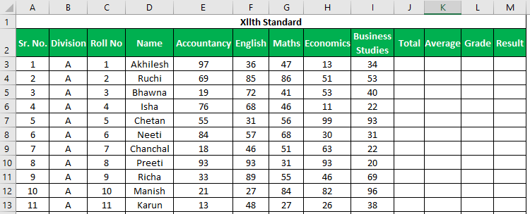
We want to find the total marks scored, an average of marks (this will also help us to give students grades), and a result that whether the student is passed or failed.
#1 – SUM Function
To find out the total, we will use the SUM
The syntax for the SUM in excel is as follows:
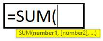
This function takes 255 numbers in this way to add. But we can also give the range for more than 255 numbers too as an argument for the function, to sum up.
There are various methods to specify numbers as follows:
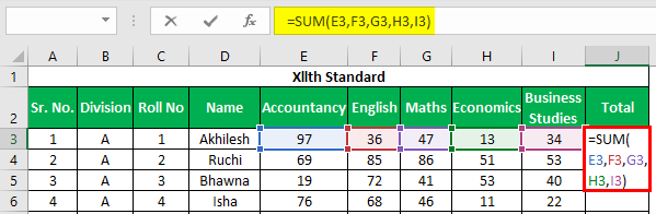
#1 – Comma Method
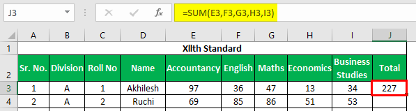
Total will be –
In this method, we use commas for specifying and separating the arguments. We have specified or selected various cells with commas.
#2 – Colon Method (Shift Method)
In this method, we have used the ‘Shift’ key after selecting the first cell (E3) and then used the Right Arrow key to select cells until I3. We can select continuous cells or specify the range with the colon manually.
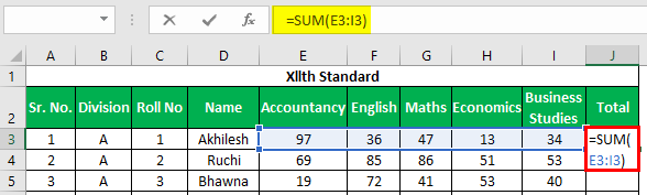
Total will be –
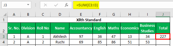
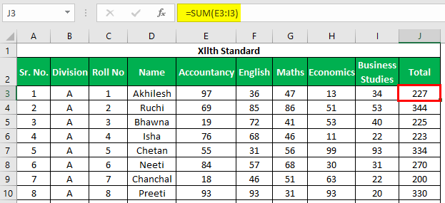
After entering the formula for the first student, we can copy down the formula using Ctrl+D as a shortcut key after selecting the range with the first cell at the top so that this formula can be copied down.
Apply the above formula to all the remaining cells. We get the following result.
#2 – AVERAGE Function
For calculating Average Marks, we will use the AVERAGE function. The syntax for the AVERAGE function is the same as the SUM function.
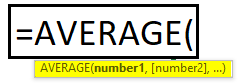
This function returns the average of its arguments.
We can pass arguments to this function in the same way as we pass arguments to the SUM function.
For evaluating the average in the excel mark sheet, we will use the AVERAGE function in the following way. We will select marks scored by a student in all 5 subjects.
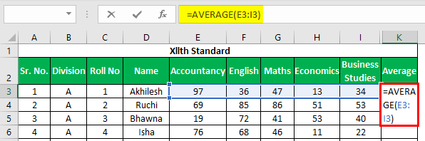
The average will be –
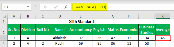
We will use Ctrl+D to copy down the function.
Apply the above formula to all the remaining cells. We get the following result.
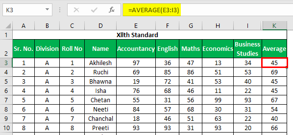
As we can see that we have got values in decimal for average marks, which doesn’t look good. Now we will use the ROUND function to round the values to the nearest integer.
#3 – ROUND Function
This function is used to round the values to the specified number of digits.
The syntax for the ROUND function in excel is as follows:
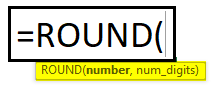
Arguments Explanation
- Number: For this argument, we need to provide the number which we want to round. We can give reference to the cell containing a number or specify the number itself.
- Num_digits: In this argument, we specify the number of digits which we want after the point in the number. If we want a pure integer, then we specify 0.
Let us use this function in the excel mark sheet. We will wrap up the AVERAGE function with the ROUND function to round the number, which will be returned by the AVERAGE function.
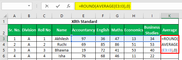
We have used the AVERAGE function for number argument and 0 for num_digits.
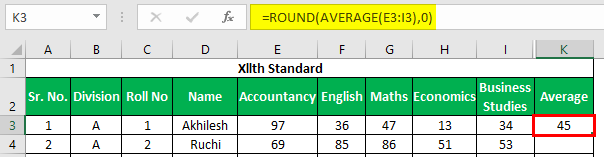
After pressing Enter, we will get the desired result, i.e., number with no decimal digit.
The average will be –
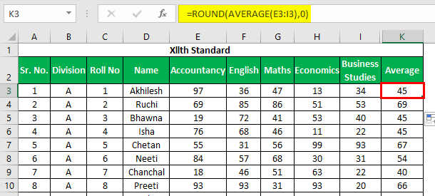
Apply the above formula to all the remaining cells. We get the following result.
#4 – IF Function
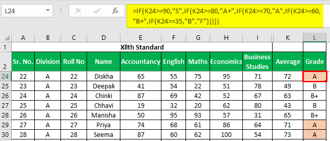
Now to find out the grade, we have the following criteria.
- If the student has scored average marks greater than or equal to 90, then Student will get grade S
- If the student has scored average marks greater than or equal to 80, then Student will get a grade A+
- If the student has scored average marks greater than or equal to 70, then Student will get a grade A
- If the student has scored average marks greater than or equal to 60, then Student will get a grade B+.
- If the student has scored average marks greater than or equal to 35, then Student will get a grade B
- If the student has scored average marks less than 35, then Student will get grade F.
To apply these criteria, we will use the IF function in excel multiple times. This is called NESTED IF in excel, also as we will use the IF function to give an argument to the IF function itself.
We have used the following formula to evaluate grade in the excel mark sheet.
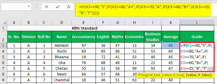
Let us understand the logic applied in the formula.
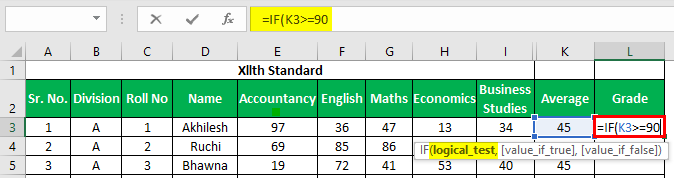
As we can see that for ‘logical_test,’ which is the criterion, we have given a reference to K3 cell containing AVERAGE of marks and have used logical operators, which is ‘Greater Than’ and ‘Equal To’ and then compared the value with 90.
It means if the average marks scored by the student is greater than or equal to 90, then write the value which we will specify in the ‘value_if_true’ argument and if this criterion is not satisfied by the average marks, then what should be written in the cell as ‘Grade,’ that we will specify for ‘value_if_false’ argument.
For the ‘value_if_true’ argument, we will specify text (Grade) within double quotes, i.e., “S.”
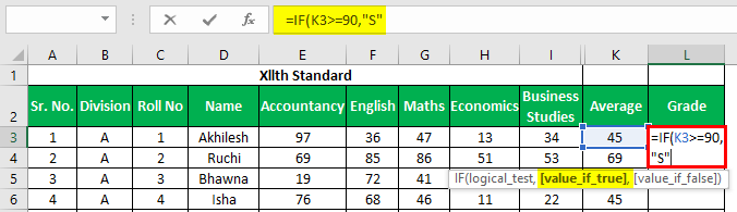
For the ‘value_if_false’ argument, we will again start writing the IF function as we have many more criteria and the corresponding grade to assign if this criterion is not satisfied.
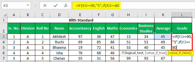
Now we have started writing the IF function again for the ‘value_if_false’ argument and specified the criteria to compare average marks with 80 this time.
The result will be –
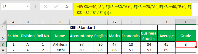
If average marks are greater than or equal to 70 but less than 80 (first IF function criteria), then Student will get an ‘A’ grade.
In this way, we will apply the IF function in the same formula for 5 times, as we have 6 criteria.
Make sure as we have opened brackets for, IF function 5 times, we need to close all brackets.
# 5 – COUNTIF
For finding out Result whether a student is “PASSED” or “FAILED,” we have to apply the following criteria.
- If the student has scored greater than 200 as total marks and scored greater than 33 in all subjects, then the student is PASSED.
- If a student has scored less than 33 in 1 or 2 subjects and total marks are greater than 200 then the student has got ER (Essential Repeat).
- If the student has scored less than 33 in more than 2 subjects or less than or equal to 200 as total marks, then the student is FAILED.
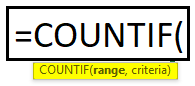
As we need to evaluate a number of subjects in which student has scored less than 33, we need to use the COUNTIF function, which will count numbers based on the specified criterion.
The syntax for the COUNTIF function is as follows:
Arguments
- Range: Here, we need to give reference to the cells containing a number to compare the criterion with.
- Criteria: To specify the criterion, we can use logical operators so that only those numbers will be counted, which will satisfy the criterion.
AND Function
The syntax for AND function excel is as follows:
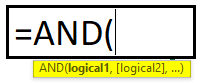
In the AND function, we specify the criteria. If all the criteria are satisfied, then only TRUE comes. We can specify up to 255 criteria.
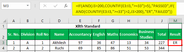
The formula which we have applied is as follows:
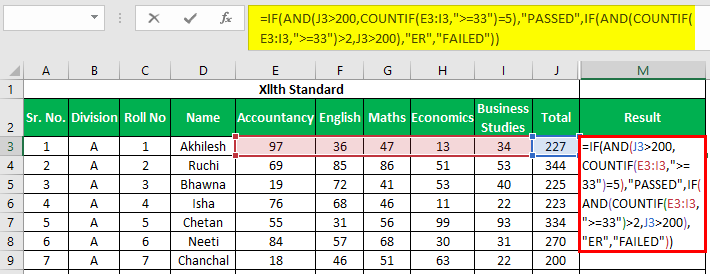
As this can be seen, we have used the AND function inside the IF function to give multiple criteria and the COUNTIF function inside the AND function to count the number of subjects in which student has scored greater than or equal to 33.
The result will be –
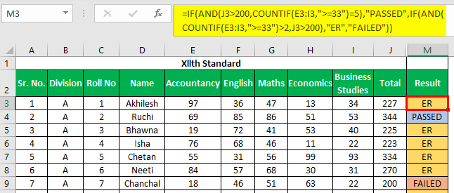
Apply the above formula to all the remaining cells. We get the following result.
Things to Remember about Marksheet in Excel
- Make sure to close the brackets for the IF function.
- While specifying any text in the function, please use double quotes (” “) as we have used while writing “Passed,” “Failed,” “ER,” etc.